3
Lesson 2: Getting the data you want

It will probably take you about 30 minutes to complete this lesson.

In lesson 1 you learned about the Discoverer workarea and looked at the Video Tutorial Workbook. In this lesson you will create your own workbook and learn how to use Discoverer's analysis tools to analyze worksheet data.

This lesson consists of the following exercises:

• "Exercise 1: Specifying default settings for your worksheets"

• "Exercise 2: Creating a new workbook"

• "Exercise 3: Saving your workbook"

• "Exercise 4: Creating page items"

• "Exercise 5: Duplicating a table worksheet as a crosstab worksheet"

• "Exercise 6: Filtering data with conditions"

• "Exercise 7: Creating parameters for other users"

• "Exercise 8: Adding items to the worksheet"

• "Lesson summary"

Exercise 1: Specifying default settings for your worksheets

In this exercise, you will learn how to specify how you want worksheet data to look by changing the Discoverer default settings. For example, worksheet font sizes, background colors, and text alignment settings. The default settings that you specify become the default settings for new workbooks that you create.

To specify default settings:

1. Connect to the Video Store Tutorial database.

   Hint: See Lesson 1: "Exercise 1: Starting Discoverer Plus".

2. For now, click Cancel to close the Workbook Wizard.

3. Choose Tools | Options to display the Options dialog.

   You use the Options dialog to specify default settings for worksheets.

4. Display the Default Formats tab.

   Figure 3-1 Options dialog: Default Formats tab

   
   
   Text description of the illustration def_for.gif

5. Select Data Format in the Default Formats list, then click Change.

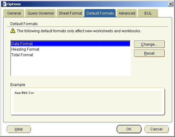
   The Data Format dialog is displayed, which you use to select font styles for data in new worksheets.

   Figure 3-2 Data Format dialog

   
   
   Text description of the illustration fontedit.gif

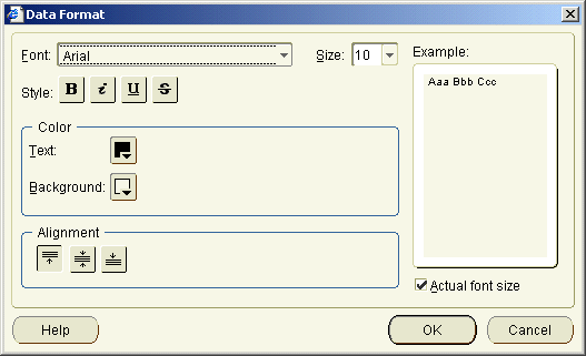
   In the Example box, you can see an example of the current font settings. This box is updated every time you make a change.

6. Click the Font drop down list and select a different font style from the font options.

7. Click the 'B' button in the Style options and notice how the example text changes to bold.

8. Choose a font size that you like from the Size drop down list.

9. Choose a text color and a background color from the Color options.

10. When you have finished, click OK to save the details and close the Data Format dialog.

11. Click OK to close the Default Formats dialog.

    Note: You can make changes to the layout of your workbooks later, using the Edit worksheet: Format tab. For example, you might want to change the format of worksheet currency (see screenshot below).

    Figure 3-3 Format data dialog: Number tab

    
    
    Text description of the illustration form_num.gif

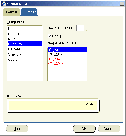
Having specified default settings for worksheets, you are now ready to create a worksheet in a Discoverer workbook.

Exercise 2: Creating a new workbook

In this exercise you will put aside the tutorial workbook Video Tutorial Workbook, and create our own workbook.

Using Discoverer's Workbook Wizard, you will select items from the video store database that you want to display in your workbook.

To create a new workbook:

1. Choose File | New to display the Workbook Wizard: Create Workbook dialog.

   Figure 3-4 Workbook Wizard: Create Workbook dialog

   
   
   Text description of the illustration ww1.gif

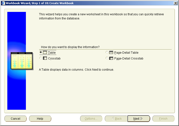
   The Worksheet Wizard: Create Workbook page enables you to specify a worksheet style. The easiest way to display your data is in a table. A table displays data in columns with column headings.

2. Select the Table radio button to select the table layout.

3. Click Next to display the Workbook Wizard: Select Items dialog.

   Figure 3-5 Workbook Wizard: Select Items dialog

   
   
   Text description of the illustration ww2.gif

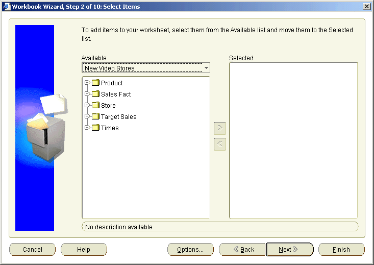
   The Workbook Wizard: Select Items dialog enables you to specify what data you want in your report.

4. Choose Video Store Tutorial from the Available drop down list.

   The options that you see in the Available drop down list are different parts of your organization's database that the Discoverer manager has defined for you. These parts of your organization's database are called business areas.

   Business areas contain data for a specific area of interest. For example, an Accounts Payable business area, a Sales business area, and an Operations business area.

   The item navigator box below the Available list displays folders and items in the Video Store Tutorial business area.

5. In the item navigator box, click the + symbol next to the Video Analysis Information folder to expand the folder.

   Figure 3-6 Workbook Wizard: Select Items dialog showing Video Analysis Information folder

   
   
   Text description of the illustration ww2a.gif

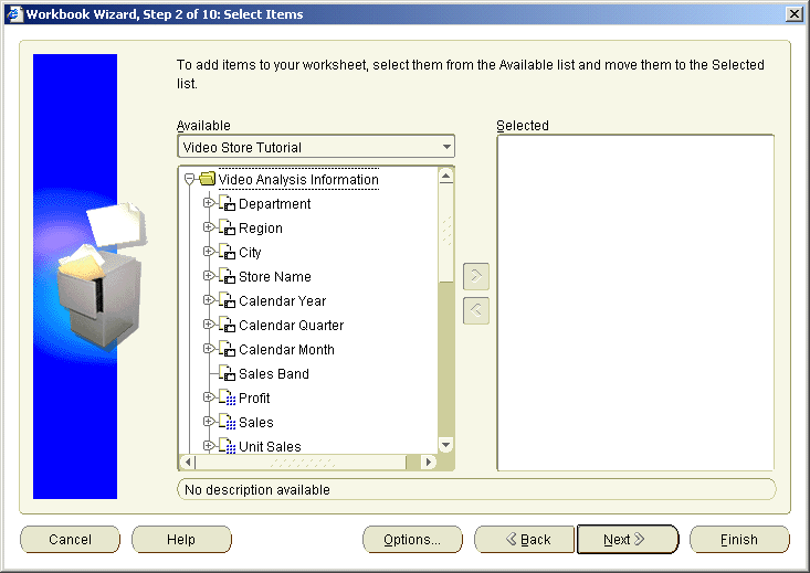
   The Video Analysis Information folder expands to show a list of items contained in this folder. For example, the first item in the list, Department, contains data about the departments in the video stores.

   Hint: Click the + and - symbols to expand and collapse folders and items.

6. Move the Department item from the Available list to the Selected list.

   Hint: To add an Item, you can either drag-and-drop it to the Selected list, or click the right arrow button.

7. Click the + symbol next to the Region item to expand the item.

   Notice that there are three regions: Central, Eastern, and Western. You can select regions individually, or select all regions available.

8. Move the Region item from the Available list to the Selected list.

   Notice that you have selected all three regions.

9. In the Available list, click the + symbol next to the Profit item so that Profit expands to show a list of additional items.

10. Move the Profit SUM item from the Available list to the Selected list.

    For numeric data like sales, costs, and profits, Discoverer provides you with a choice of aggregations (e.g. sum, average, minimum). For example, if you want to know the total profit for a particular region, select SUM. If you want to know the average profit for the same region, select AVG.

11. Move the Calendar Year item from the Available list to the Selected list.

    You should now have the following items in the Selected list:

    • Department

    • Region

    • Calendar Year

    • Profit SUM

12. Click Next to display the Workbook Wizard: Table Layout dialog.

    Figure 3-7 Workbook Wizard: Table Layout dialog

    
    
    Text description of the illustration ww3.gif

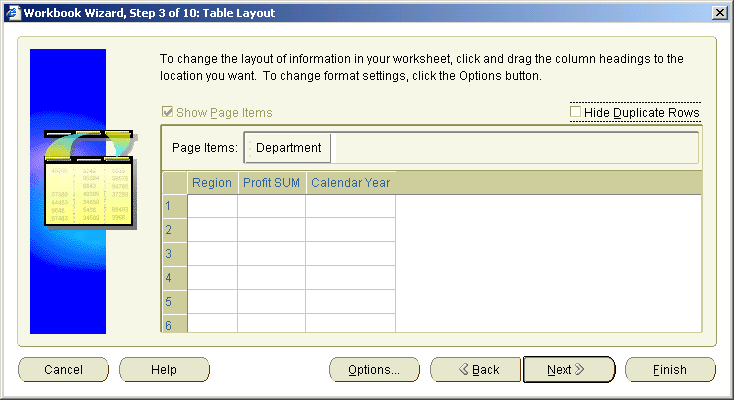
    You can see that Department is in the Page Items area. Region, Profit SUM, and Calendar Year are in the body of the worksheet.

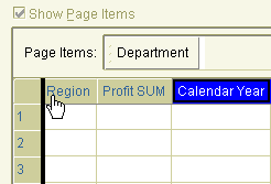
    Here, you want to re-order the items to display the Calendar Year item to the left of the Region item.

13. Drag and drop the Calendar Year item to the left of the Region item.

    A black bar between the columns indicates where the item will be positioned when you release the cursor.

    Figure 3-8 Re-ordering worksheet items

    
    
    Text description of the illustration chg_lay1.gif

    Figure 3-9 Reordered worksheet items

    
    
    Text description of the illustration chg_lay2.gif

14. Click Next to display the Worksheet Wizard: Format page.

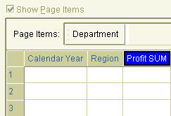
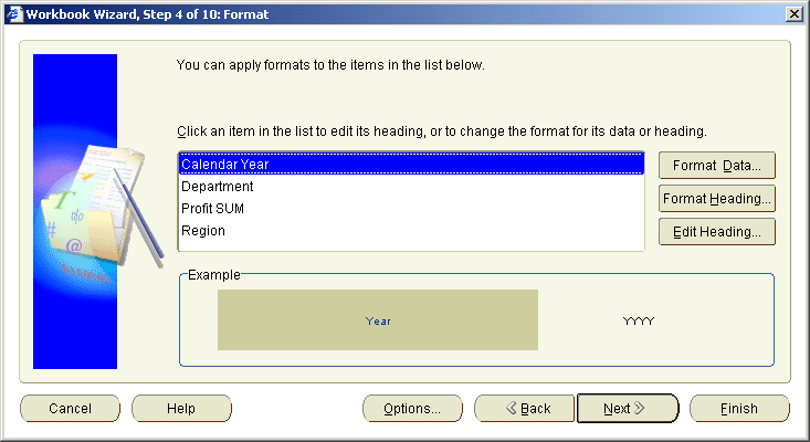
    Because you specified default settings earlier, you will leave the format unchanged.

    Figure 3-10 Workbook Wizard: Format tab

    
    
    Text description of the illustration chg_lay3.gif

15. Click Next to display the Worksheet Wizard: Conditions page.

    Figure 3-11 Conditions list

    
    
    Text description of the illustration wb5.gif

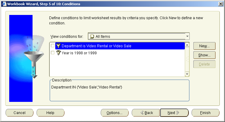
    You want to display only data from the Video Rental or Video Sale departments on the new worksheet.

16. Select the Department is Video Rental or Video Sale check box.

    Figure 3-12 Conditions list

    
    
    Text description of the illustration wb5a.gif

17. Click Finish to close the Workbook Wizard.

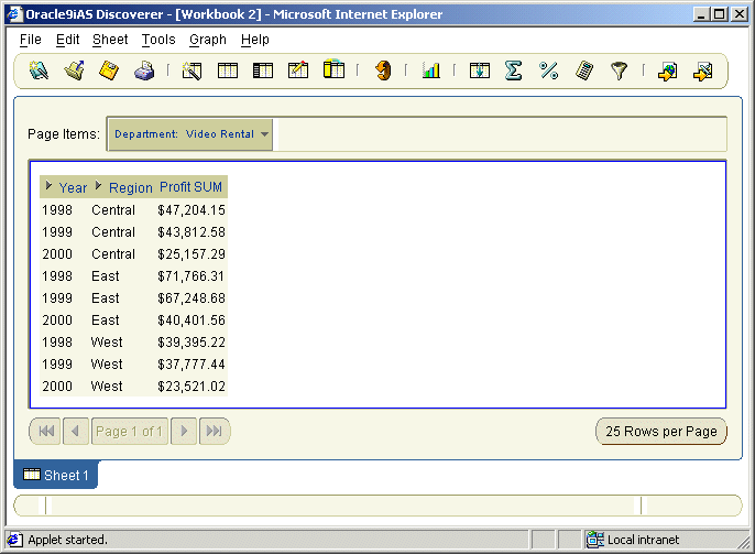
    A new worksheet is displayed, called Sheet 1. Sheet 1 contains the data for the items you selected. Notice that the item layout matches the layout that you specified in the Workbook Wizard.

    Figure 3-13 Sheet 1 worksheet

    
    
    Text description of the illustration sheet1.gif

Having created a worksheet in Discoverer, you are now ready to save the workbook in the database.

Exercise 3: Saving your workbook

In this exercise you will learn how to save workbooks in the database.

Note: The Discoverer manager must grant you the privilege to save workbooks in the database.

1. Choose File | Save As to display the Save workbook to Database dialog.

2. Enter a name for the new workbook in the New name field.

   For example, 'My tutorial workbook'.

   Figure 3-14 Save Workbook to Database dialog

   
   
   Text description of the illustration savewb.gif

3. Click Save to save the details and close the Save Workbook to Database dialog.

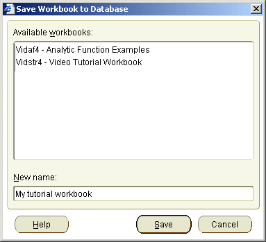
Having saved your workbook, you are now ready to begin customizing the workbook for easier analysis.

Exercise 4: Creating page items

In this exercise you will learn how to create a page item using Discoverer's pivoting capabilities to make your worksheet easier to analyze.

In your worksheet, the Department item is displayed in the Page Items area. This means that the worksheet displays data for one department at a time. You want to display data for one region at a time, so that you can analyze data for all departments in particular regions.

To create a page item:

1. Choose Sheet | Edit Sheet to display Edit worksheet dialog.

   Notice that the tabs on the Edit worksheet dialog match the pages on the Workbook Wizard. This enables you to go back to any aspect of a worksheet and change something.

2. Display the Table Layout tab.

   Figure 3-15 Edit Worksheet: Table Layout tab

   
   
   Text description of the illustration tab_lay.gif

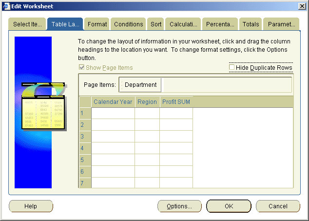
   The Edit Worksheet: Table Layout tab enables you to create page items, and re-arrange worksheet items. If you rearrange worksheet items, you do not affect the data itself.

   Notice that the Show Page Items check box is selected, which means that the area is active.

3. Drag the Department item down into the main body of the table to the right of the Calendar Year item.

   Figure 3-16 Moving the Department item from the Page Items area to the body of the worksheet

   
   
   Text description of the illustration page1.gif

4. Drag the Region item into the Page Items area next the Department item.

   Figure 3-17 The Worksheet layout tab

   
   
   Text description of the illustration page3.gif

5. Click OK to save the details and close the Edit Worksheet dialog.

   Figure 3-18 Worksheet with Region displayed in the Page Items area

   
   
   Text description of the illustration page2.gif

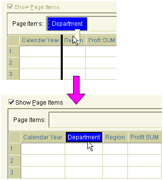
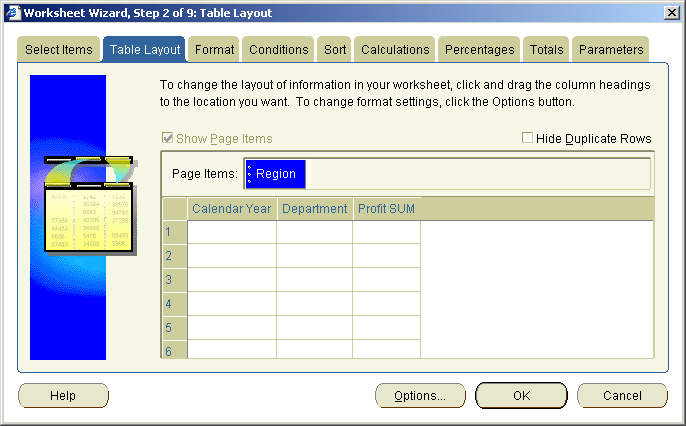
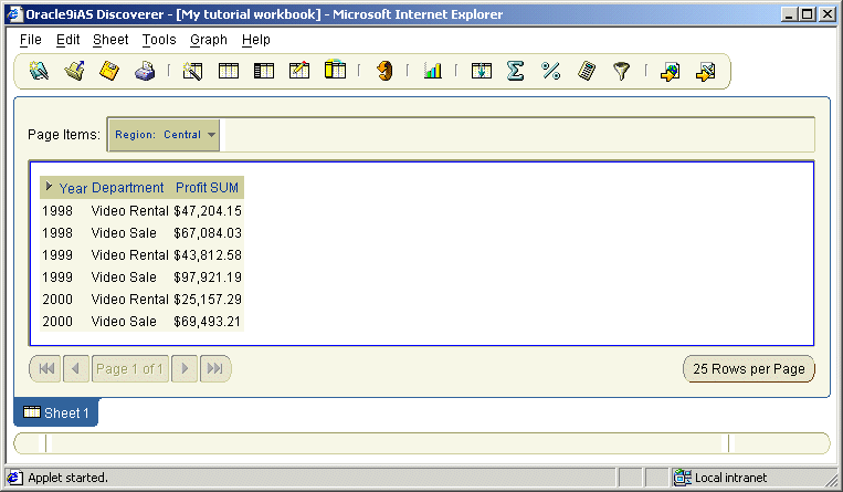
   Notice that the Region item is displayed in the Page Items area. The Department Item is now displayed between the Year and Profit SUM columns.

6. Select the East region from the Region drop down list.

   Notice how the worksheet is refreshed to display data for the East region.

7. Choose File | Save to your work.

   Having rearranged your worksheet for easier analysis, you are now ready to create a crosstab worksheet to enable more advanced analysis.

Exercise 5: Duplicating a table worksheet as a crosstab worksheet

In this exercise you will learn how to quickly create a new worksheet based on an existing worksheet.

Here, you get a new worksheet containing the same items as in the table worksheet, but in crosstab format. A crosstab relates two sets of data and then summarizes their interrelationship in terms of a third set of data.

For example, a typical crosstab for the video stores shows the monthly profit for each region, organized by department. In other words, there are three sets of data: total sales, region, and department. By duplicating your table as a crosstab, Discoverer calculates a subtotal of the profit for each region, as shown below.

Figure 3-19 Crosstab worksheet example

Text description of the illustration ct.gif

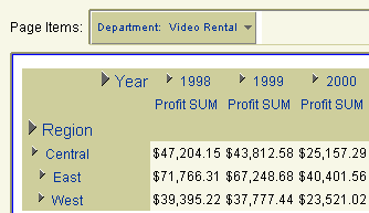
Notice that the crosstab worksheet contains additional profit sub-totals for each region in each year. Notice also that the Region item is now positioned on the left axis, with regions displayed on the left hand side as row headings.

To duplicate the table worksheet as a crosstab worksheet:

1. Choose Sheet | Duplicate as Crosstab.

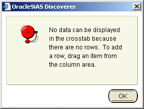
   Discoverer displays an alert dialog to let you know that you must have rows defined in a crosstab. Rows on crosstabs are left axis items.

   Figure 3-20 Discoverer alert dialog

   
   
   Text description of the illustration warn.gif

2. Click OK to display the Edit Worksheet: Crosstab Layout tab.

   Figure 3-21 Duplicate as Crosstab dialog: Crosstab Layout tab

   
   
   Text description of the illustration dup1.gif

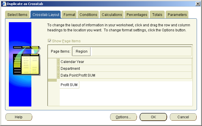
   Notice that there are three items on the top axis (Calendar Year, Department, and Data Point:Profit SUM), but that there a now items on the left axis. Remember that on a crosstab worksheet you need to have items on both the top axis and left axis.

3. Drag the Region item from the Page Items area to the left axis.

   Figure 3-22 Dragging the Region item from the Page Items area to the left axis

   
   
   Text description of the illustration dup2.gif

4. Drag the Department item to the Page items area.

   Figure 3-23 Dragging the Department item to the Page Items area

   
   
   Text description of the illustration dup3.gif

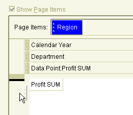
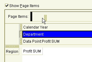
   The Department item should now be positioned in the Page Items area, and the Region item should be positioned on the left axis (see figure below).

   Figure 3-24 Worksheet layout after items have been positioned

   
   
   Text description of the illustration dup4.gif

5. Click OK to save the details and close the Edit Worksheet: Crosstab Layout tab.

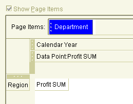
   When Discoverer displays the new worksheet, notice that the crosstab is organized by Region on the left axis, and Year on the top axis.

   Figure 3-25 Rearranged worksheet

   
   
   Text description of the illustration ct2.gif

   Having learned how to change the layout of worksheets create table and crosstab worksheets, you are now ready to learn how to filter worksheet data using conditions.

Exercise 6: Filtering data with conditions

In this exercise you will learn how to use worksheet conditions to display specific data.

Some video stores show larger profits than others. What factors cause some stores to earn more profit than others? If you are getting data from a very large database, the amount of data you get could be so large that you would have difficulty finding the answer to that question. If you are interested in analyzing only the stores with the highest profits, how could you reduce the amount of data you get from the database? For example, you might ask 'Which stores have annual profits greater than $20,000?'.

Discoverer provides you with worksheet items called conditions to reduce the amount of data you get from the database. Conditions enable you to focus on data that you are interested in and ignore data that you are not interested in.

To filter data with conditions:

1. Display the Sheet 1 worksheet.

   Figure 3-26 Sheet 1 worksheet

   
   
   Text description of the illustration sheet3.gif

2. Choose Tools | Conditions to display the Edit worksheet dialog.

3. Display the Conditions tab.

   Figure 3-27 Edit Worksheet dialog: Conditions tab

   
   
   Text description of the illustration cond1.gif

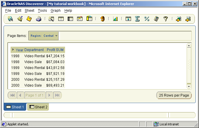
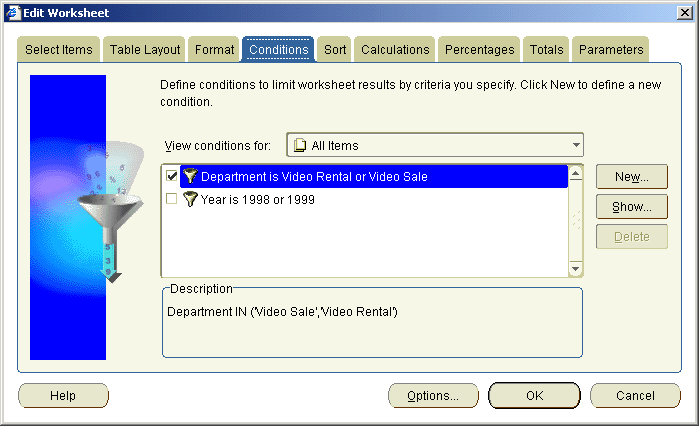
   Notice that two conditions already exist. They were created for you by the Discoverer manager.

   You want to limit the data to only Regions with annual profit greater than 50,000 dollars. To do this, you create a new condition.

4. Click New to display the New Condition dialog.

   Figure 3-28 New Condition dialog

   
   
   Text description of the illustration cond2.gif

5. If the Generate name automatically check box is not selected, select this check box.

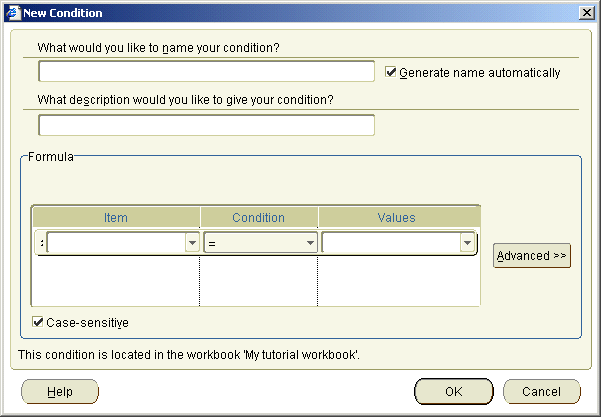
   Discoverer creates a condition name for you.

6. Type Regions with annual profits greater than $50,000 in the What description would you like to give your condition? field.

   This description is displayed in the Conditions tab, and helps other Discoverer users understand what the condition does.

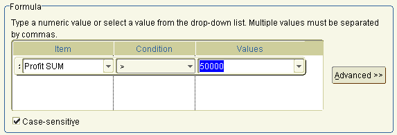
   Look at the Formula box. This is where you build the condition. Discoverer displays any data that matches the condition criteria and ignores data that does not match the condition criteria.

   In this example, you want to display only data about regions with profits greater than 50,000 dollars.

7. In the Item field, select Video Analysis Information.Profit SUM.

8. In the Condition field, select the 'greater than' symbol [>].

9. In the Value field, enter 50000.

   Figure 3-29 The Formula box with the condition details entered

   
   
   Text description of the illustration cond5.gif

10. Click OK to save the details and return to the Conditions tab.

    Figure 3-30 Edit Worksheet dialog: Conditions tab

    
    
    Text description of the illustration cond3.gif

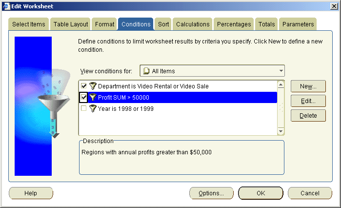
    Notice the name of your new condition: Profit SUM > 50000. This is the condition name that Discoverer generated automatically for you. The Description box below contains the additional information that you entered when you created the condition. Notice that the new condition is selected by default. If you want to turn off the condition, clear this check box.

11. Click OK to close the Conditions tab and display the worksheet.

    Discoverer sends a new query to the database and shows you the new results in the worksheet. Notice that you now have less data. Only regions with annual profits greater than 50,000 dollars are shown.

    Figure 3-31 Worksheet with Profit SUM > 50000 condition applied

    
    
    Text description of the illustration cond4.gif

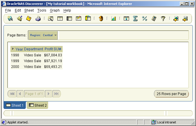
    As you can see, in the Central region, only the Video Sale Department generated profits in excess of $50,000 (in 1998, 1999, and 2000). You could now print a report of this data or mail it as a HTML file.

    Having produced a report, you now want to turn off the condition 'Profit SUM > 50000' in order to display all of the data once more. To do this, you turn off the condition 'Profit SUM > 50000' that you have just created. You can always turn it back on again later if required. Alternatively, you could delete the new condition permanently.

12. Choose Tools | Conditions, then clear the 'Profit SUM > 50000' condition check box.

13. Click OK to return to the worksheet.

    Notice how you can see all of the data, not just those regions with profits greater than $50,000.

    Having learnt how to filter data in a worksheet, you are now ready to learn how to apply dynamic user input to worksheets using parameter items.

Exercise 7: Creating parameters for other users

In this exercise you will learn how to create worksheet parameters to provide dynamic input to conditions.

Sometimes you might want other Discoverer uses to open your workbook, but only to look at specific areas of data. For example, users might typically want to look at only data for a particular month, such as January or February.

Discoverer provides you worksheet items called parameters, which enable worksheet users to provide dynamic input to conditions, calculations, and other worksheet items.

You will create a new parameter that asks worksheet users which year they want to look at. Every time the workbook is opened or refreshed, Discoverer will prompt worksheet users to specify which year they want to analyze.

Hint: Before you start this exercise, make sure that you have turned off the condition Profit SUM > 50000, (see final step in "Exercise 6: Filtering data with conditions").

To create a parameter:

1. Choose Tools | Parameters to display the Edit worksheet dialog.

2. Display the Parameters tab.

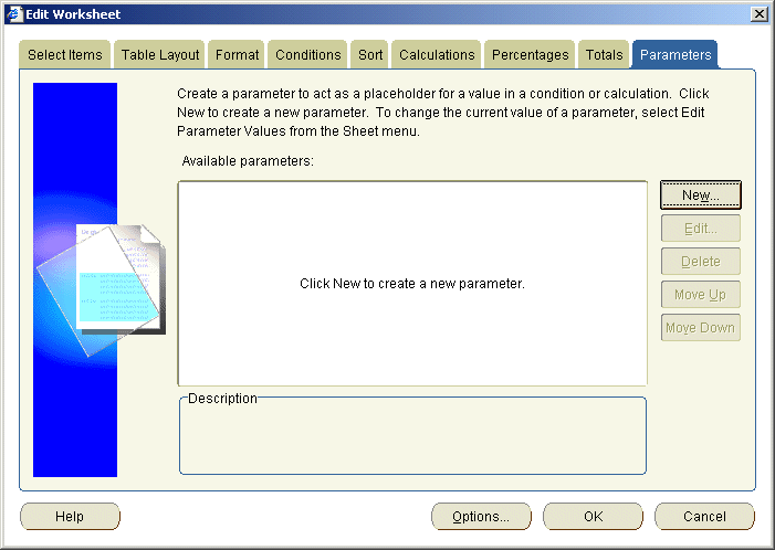
   The Parameters tab lists existing parameters available to the workbook.

   Figure 3-32 Edit Worksheet dialog: Parameters tab

   
   
   Text description of the illustration param1.gif

3. Click New to display the New Parameter dialog.

   Figure 3-33 New Parameter dialog

   
   
   Text description of the illustration param2.gif

4. In the What do you want to name this parameter? field, enter 'Choose a Year'.

5. In the Which Item do you want to base this parameter on? field, select Video Analysis Information.Calendar Year.

6. In the What prompt do you want to show other users? field, enter 'Please select which year(s) you want to analyze'.

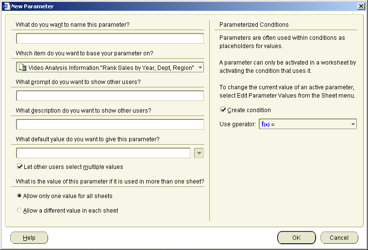
   This prompt will be displayed whenever the worksheet is opened or refreshed.

7. In the What description do you want to show other users? field, type 'Restrict the workbook to one or more years'.

   This description will is displayed whenever the worksheet is opened or refreshed to help worksheet users understand what values to select.

8. Click the What default value do you want to give this parameter? drop down list and select 2000.

   This default parameter value will be selected whenever the worksheet is opened or refreshed. This value is typically the most commonly selected value or the first value used (e.g. January in a series of months).

9. Select the Let users select multiple values check box.

   Selecting the Let users select multiple values check box enables you to display data relating to more than one value. For example, you might select January, February, and March to analyze data for all three months, rather than just for January.

10. Leave the other default values unchanged (see figure below).

    Figure 3-34 The New Parameter dialog with the values selected

    
    
    Text description of the illustration param6.gif

11. Click OK to return to the Parameters dialog.

    Figure 3-35 Edit Worksheet dialog: Parameter tab

    
    
    Text description of the illustration param3.gif

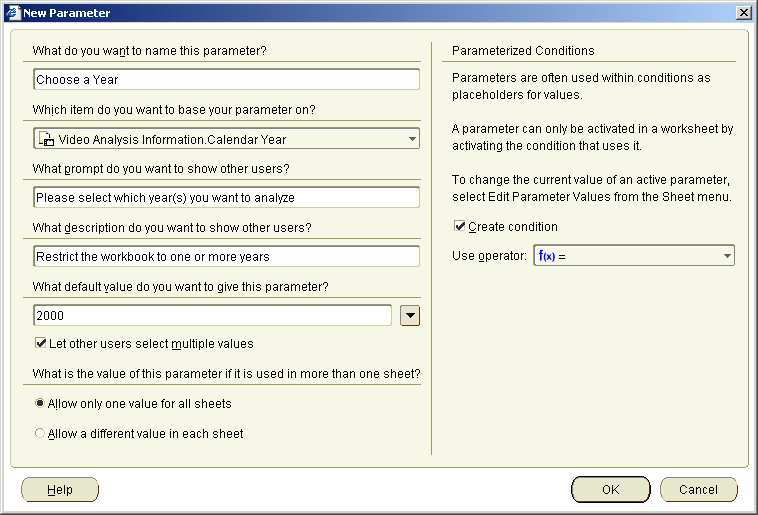
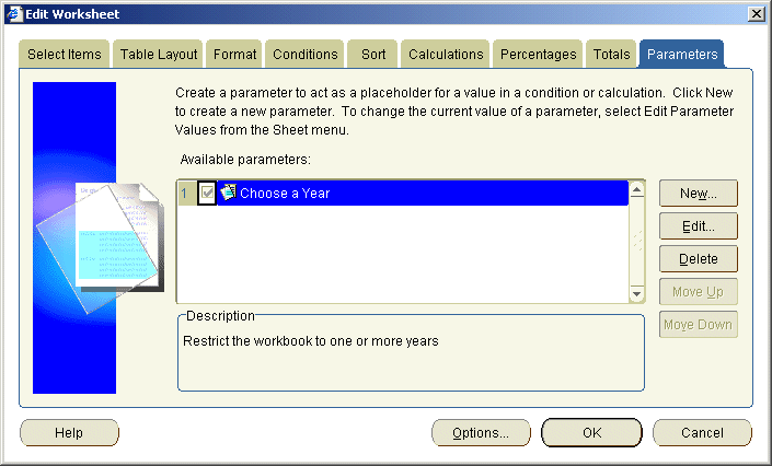
    Notice that your new parameter, called Choose a Year, is displayed turned on by default (i.e. its check box is selected). Look at the Description box at the bottom. The description that you entered is displayed (i.e. 'Restrict the workbook to one or more Years').

12. Click OK to close the Parameters tab and return to the worksheet.

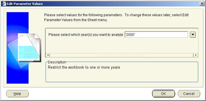
    Because the new parameter is turned on, the Edit Parameter Values dialog is displayed and displays the prompt 'Please select which year(s) you want to analyze'.

    Figure 3-36 Edit Parameter Values dialog

    
    
    Text description of the illustration param4.gif

13. Leave the default value (2000) unchanged and click OK.

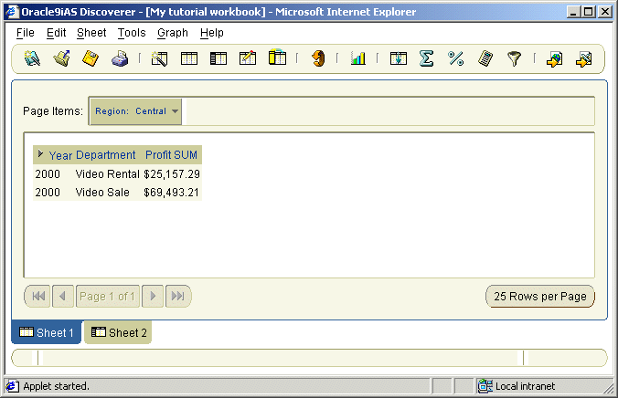
    Discoverer refreshes the worksheet. Only data for the year 2000 is displayed.

    Figure 3-37 Sheet 1 worksheet with parameter applied

    
    
    Text description of the illustration param5.gif

    Because you selected the Create condition check box when you created the parameter, you can turn this parameter value on and off using the Conditions dialog.

14. To turn this parameter off, choose Tools | Conditions to display the Conditions tab, then clear the Calendar Year = :Choose a Year check box.

15. Click OK to display the worksheet.

    Note: Notice that in the condition, the Choose a Year argument is prefixed with a colon ':'. The colon indicates that the value is dynamically set by a parameter. In other words, the colon indicates that the value can change every time the worksheet is opened or refreshed when the parameter value is updated.

Exercise 8: Adding items to the worksheet

In this exercise you will learn how to add new data items to the worksheet to enable you to analyze data in a new way.

Now that you have begun to organize your data for analysis, you realize that you need more information in your report. You know the profit for each region, but you would also like to compare the profit with sales amounts. You therefore need to add the Sales item to the worksheet.

To add an item to the worksheet:

1. Display the tabular worksheet by clicking the Sheet 1 tab at the bottom of the workbook.

   Figure 3-38 Sheet 1 worksheet

   
   
   Text description of the illustration sheet3.gif

2. Choose Sheet | Edit Sheet to display the Edit worksheet dialog at the Select items tab.

   Figure 3-39 Select Items tab

   
   
   Text description of the illustration add1.gif

3. In the Available list, click the [+] next to the Video Analysis Information folder to expand the folder.

4. From the list of items, move the Sales SUM item from the Available list to the Selected list.

   Figure 3-40 Moving the Sales SUM item to the Selected list

   
   
   Text description of the illustration add2.gif

5. Click OK to close the Edit worksheet dialog.

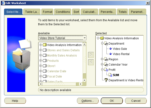
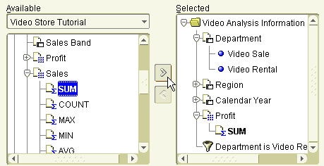
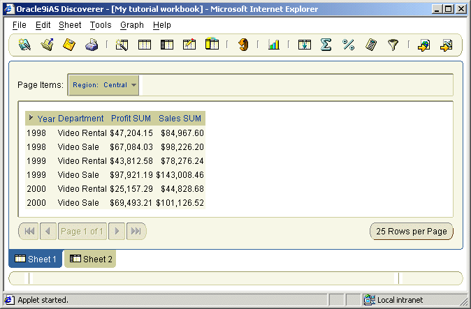
Your worksheet now contains the new item Sales SUM. You can now analyze how Sales figures relate to Profit figures.

Figure 3-41 Discoverer worksheet with additional Sales SUM item

Text description of the illustration sales.gif

Lesson summary

In this lesson you:

• defined new default worksheet settings

• created your own worksheets in a new workbook

• organized items on the worksheet to make them easier to analyze

• created a new worksheet by duplicating an existing worksheet

• reduced the amount of data in a worksheet using conditions and parameters enabling you to publish interactive reports

• added new items to your new workbook

Now you are ready to find out how easy it is to create powerful reports in Discoverer, described in "Lesson 3: Analyzing your data".

Frequently asked questions

How does changing default settings affect existing workbooks?

Default settings only affect new workbooks that you create. Changing default settings does not change the layout of existing workbooks or workbooks that were created by other Discoverer Plus users. (To change the format of existing worksheets, choose Sheet | Format.)

Where will you find the name of your workbook on the workbook itself?

The workbook's name is displayed at the top of the workbook, in brackets. For example, [Video Tutorial Workbook].

What is the difference between a condition and a parameter?

Conditions enable you to filter data in the same way each time a workbook or worksheet is opened or refreshed.

Parameters enable you to filter data in a different way each time the workbook or worksheet is opened or refreshed. Parameters also enable you to provide input values to calculations. For more information, see "Glossary".

How do you turn conditions on and off?

From the Tools menu, choose Conditions. In the Conditions dialog, you see a list of conditions that already exist. A selected check box next indicates that a condition is turned on (i.e. active).

For example, the 'Sales by Region' worksheet contains data that answers the question (query) 'What are my company's sales for the Eastern, Central, and Western regions?'.

What is the difference between an item and a page item?

Items are different types of information stored in a folder. For example, if a products folder contains reference numbers, descriptions, and the price of each product, the items in the products folder are reference number, description, and price. Items appear as worksheet columns and rows.

In Lesson 2 you will learn how to select Items from the database with the Workbook Wizard. On a worksheet. In Lesson 3 you will learn how to rearrange Items on a worksheet.

A page item is a filtering item located above a worksheet in the Page Items area. Page items enable you to look at one area of information at a time. For example, if an item called Month is placed in the Page Items area, you might select January from the page item drop down list to produce a January report, then select February to produce a February report and so on.

In Lesson 3, "Exercise 2: Pivoting rows and columns" you will learn how to create Page Items and how to switch between them.

What is the Workbook Wizard?

The Workbook Wizard is a Discoverer tool that helps you create new workbooks or worksheets. The Workbook Wizard takes you step-by-step through the worksheet creation process. In Lesson 2, you will use the Workbook Wizard to create a new worksheet.

Discoverer also provides wizards to help you print and export Discoverer data.