Segment Tree

The Segment Tree is a binary tree built on top of an array, where every node stores the answer for a contiguous range of positions. It is the Swiss army knife of range queries: the same skeleton answers range sums, range minimums, counts, and many more queries, while the array changes. Its operations usually take logarithmic time.

We start from the problem already solved by the Fenwick tree, so we can compare the two, and then we move to problems that the Fenwick tree cannot handle.

Notice that, differently from the Fenwick tree notes, here we use a zero-based indexing.

Throughout these notes we use the following array as a running example, for every problem we discuss.

Its values are non-negative and some of them repeat: we will need both properties later.

The Segment Tree

The Segment Tree is a balanced binary tree whose leaves are the entries of \(A,\) from left to right. Each node covers the range of positions of the leaves below it, and it stores the answer of the query on that range. For our problem, a node covering the range \([l, r]\) stores the sum \(A[l] + A[l+1] + \cdots + A[r].\)

The root covers the whole array \([0, n-1].\) A node covering \([l, r],\) with \(l < r,\) has two children. If \(m = \lfloor (l+r)/2 \rfloor,\) the left child covers \([l, m]\) and the right child covers \([m+1, r].\) A node covering a single position \([i, i]\) is a leaf, and it stores \(A[i].\)

The figure below shows the Segment Tree of our running example. Next to every node we report its range.

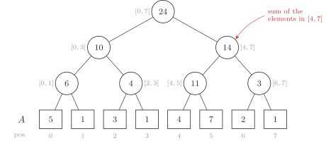
Since the range of a node is split in two halves, the height of the tree is \(\lceil \log n \rceil.\) The tree has \(n\) leaves and \(n-1\) internal nodes, so \(2n-1\) nodes in total, and it uses linear space. When \(n\) is not a power of \(2,\) the two halves of a node may differ by one, and some leaves are one level higher than others.

Observe that the value of an internal node is the sum of the values of its two children. For example, the node \([4,7]\) stores \(14 = 11 + 3.\) This gives us the construction: we build the two children recursively, and then we set the node to the sum of their values. A leaf \([i, i]\) is set to \(A[i].\) We do a constant amount of work per node, so the construction takes \(\Theta(n)\) time. This is better than starting from an array of zeros and performing \(n\) add operations, which takes \(\Theta(n \log n)\) time.

Performing an add operation

Consider the operation add(i, v). Which nodes must change? Exactly the nodes whose range contains position \(i.\) These are the leaf \(i\) and all its ancestors, which are the nodes on the path from the root to the leaf \(i.\)

We go down from the root to the leaf \(i,\) choosing at every node the child whose range contains \(i.\) We add \(v\) to the leaf. Then, on the way back up, we recompute every node on the path from the values of its two children, exactly as in the construction. Only one child has changed, but the other child already stores the correct value.

The figure below shows add(4, 3) on our running example. The four nodes on the path from the root to the leaf \(4\) increase by \(3.\) All the other nodes do not change, because their ranges do not contain position \(4.\)

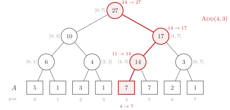
For sums we could simply add \(v\) to every node on the path. Recomputing every node from its children is the general way, and it works for every operation we will see in these notes.

The path has one node per level, so add modifies \(\Theta(\log n)\) nodes and takes \(\Theta(\log n)\) time.

Answering a range_sum query

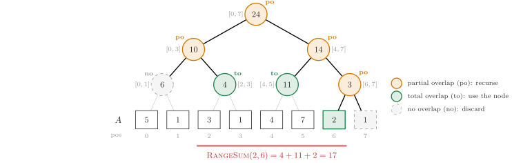
Let’s go back to the original array (without the add above) and consider the query range_sum(2, 6), whose answer is \(3+1+4+7+2 = 17.\)

The query is answered with a recursive visit that starts from the root. When the visit reaches a node covering \([l, r],\) there are three possible cases, depending on how the range of the node overlaps the query range \([i, j].\)

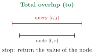
1. Total overlap (to): the query range contains the range of the node, i.e., \(i \leq l\) and \(r \leq j.\) The value of the node is exactly the contribution of this part of the array. We stop the recursion and return the value of the node.

   

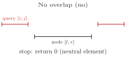
2. No overlap (no): the two ranges are disjoint, i.e., \(r < i\) or \(j < l.\) This part of the array does not contribute. We stop the recursion and return \(0.\)

   

3. Partial overlap (po): any other case. Part of the range of the node is in the query and part is not. We recurse on both children and return the sum of their results.

   

The figure below shows the visit for range_sum(2, 6). The answer is the sum of the values of the nodes with a total overlap: \([2,3],\) \([4,5]\) and \([6,6],\) that is, \(4 + 11 + 2 = 17.\) Notice that these three nodes partition the query range.

How many nodes do we visit?

Nodes with a total overlap or no overlap are cheap: they stop the recursion. The cost comes from the nodes with a partial overlap, because each of them generates two recursive calls. So, the question is: how many partial overlaps can there be?

Consider a node \([l, r]\) with a partial overlap, and let \(m\) be its middle point. What matters is the part of the query inside the node, that is, \([\max(i, l), \min(j, r)].\) There are three possibilities.

1. It is inside one half of the node. One child has no overlap, and the visit continues on the other child only.

   

2. It touches an extreme of the node, i.e., it is a suffix \([i, r]\) or a prefix \([l, j]\) of the range of the node, and it crosses the middle point. Consider a suffix \([i, r]\) with \(i \leq m.\) The right child has a total overlap and stops immediately. The left child gets again a suffix of its range. Prefixes are symmetric.

   

3. It crosses the middle point and touches no extreme: \(l < i \leq m < j < r.\) We call it a general partial overlap. The query is split into two pieces: the left child gets the suffix \([i, m]\) of its range and the right child gets the prefix \([m+1, j]\) of its range.

   

The first two possibilities are harmless: one child stops immediately, and the visit continues on the other child only. The general partial overlap is the potential source of inefficiency, because both children continue. If both children had a general partial overlap too, and their children too, and so on, the visit could reach every node of the tree. A query would then cost \(\Theta(n),\) no better than scanning the array.

Luckily, this does not happen. The children of a general partial overlap get very special query parts. Look at the node \([l, r]\) in the figure below. Its left child \([l, m]\) gets the suffix \([i, m]:\) the right extreme of its query part is anchored to the end of its range (the dot in the figure). Symmetrically, the right child \([m+1, r]\) gets the prefix \([m+1, j],\) whose left extreme is anchored to the beginning of its range.

An anchored query part can never produce a general partial overlap, because a general partial overlap touches no extreme of the node. So, even if a descendant has a partial overlap, it is one of the easy ones. Consider a node \([l, r]\) that gets a suffix \([i, r],\) i.e., a query part anchored to the end of its range. Where can its middle point \(m\) cut the query part? There are only two possibilities.

• The middle point is before the query part, i.e., \(m < i.\) The left child has no overlap and stops. The right child gets the suffix \([i, r],\) again anchored to the end of its range, and the visit continues there (with a total overlap, if \(i = m+1\)).

  

• The middle point cuts the query part, i.e., \(i \leq m.\) The right child \([m+1, r]\) is entirely inside the query, so it has a total overlap and stops. The left child gets the suffix \([i, m],\) again anchored to the end of its range, and the visit continues there.

  

The cases of a query part anchored to the beginning of the range, i.e., a prefix \([l, j],\) are symmetric. If \(j \leq m,\) the right child has no overlap and stops, and the left child continues with the prefix \([l, j].\) If \(m < j,\) the left child has a total overlap and stops, and the right child continues with the prefix \([m+1, j].\)

In both cases, one child stops and the other one gets again an anchored query part, so the same argument applies to it, all the way down. Thus, there is at most one general partial overlap. Above it, the query part is inside one half of each node, so there is a single path. Below it, there are two paths, one towards each extreme of the query, and every node on them has a partial overlap of the easy kind.

Let’s read the figure of range_sum(2, 6) in this way. The root \([0,7]\) is the general partial overlap, since \(0 < 2 \leq 3 < 6 < 7.\) The node \([0,3]\) gets the suffix \([2,3]\) of its range: its left child \([0,1]\) has no overlap, and its right child \([2,3]\) has a total overlap. The node \([4,7]\) gets the prefix \([4,6]:\) its left child \([4,5]\) has a total overlap, and the visit continues on \([6,7].\)

The figure below shows the same shape on a larger example, the query \([3, 12]\) on an array of \(n = 16\) entries. The root is the only general partial overlap. From there, two paths go down to the extremes of the query, and the total overlaps hang off these paths.

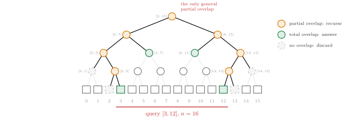
Summing up, we visit at most \(4\) nodes per level: the nodes on the (at most) two paths and at most one sibling of each of them, which has a total overlap or no overlap. Therefore, range_sum takes \(O(\log n)\) time. This is a worst-case bound: some queries are cheaper, e.g., range_sum(0, n-1) stops at the root.

Segment Tree in Rust

Here, we present a minimal Rust implementation of the Segment Tree. As in the Fenwick tree notes, we choose i64 as the type of the values. We use the same names as the text: a node covers \([l, r],\) and the query is \([i, j].\)

We store the tree in a vector, as we do for binary heaps. The root is node \(0\) and the children of node \(u\) are nodes \(2u+1\) and \(2u+2.\) The nodes do not store their ranges: the recursive functions compute them on the way down, starting from the range \([0, n-1]\) of the root.

How large must the vector be? The tree has \(2n-1\) nodes, but with this layout their indexes are not contiguous when \(n\) is not a power of \(2,\) and they may exceed \(2n-2.\) For example, for \(n = 6\) the leaf \(4\) is node \(12.\) A safe bound is \(4n.\) The tree has height \(h = \lceil \log n \rceil,\) and a heap layout of height \(h\) uses indexes smaller than \(2^{h+1}.\) Since \(2^{h} < 2n,\) the indexes are smaller than \(4n.\) There are more compact layouts, but this one is simple and good enough for us.

#[derive(Debug)]
pub struct SegmentTree {
    n: usize,
    tree: Vec<i64>,
}

impl SegmentTree {
    pub fn from_slice(a: &[i64]) -> Self {
        assert!(!a.is_empty());
        let n = a.len();
        let mut st = Self { n, tree: vec![0; 4 * n] };
        st.build(a, 0, 0, n - 1);
        st
    }

    pub fn len(&self) -> usize {
        self.n
    }

    /// A[i] += v
    pub fn add(&mut self, i: usize, v: i64) {
        assert!(i < self.n);
        self.add_rec(0, 0, self.n - 1, i, v);
    }

    /// A[i] + A[i+1] + ... + A[j]
    pub fn range_sum(&self, i: usize, j: usize) -> i64 {
        assert!(i <= j && j < self.n);
        self.range_sum_rec(0, 0, self.n - 1, i, j)
    }

    // Node u covers [l, r]; its children are 2u + 1 and 2u + 2.
    fn build(&mut self, a: &[i64], u: usize, l: usize, r: usize) {
        if l == r {
            self.tree[u] = a[l];
            return;
        }
        let m = (l + r) / 2;
        self.build(a, 2 * u + 1, l, m);
        self.build(a, 2 * u + 2, m + 1, r);
        self.tree[u] = self.tree[2 * u + 1] + self.tree[2 * u + 2]; // combine
    }

    fn add_rec(&mut self, u: usize, l: usize, r: usize, i: usize, v: i64) {
        if l == r {
            self.tree[u] += v; // the leaf of position i
            return;
        }
        let m = (l + r) / 2;
        if i <= m {
            self.add_rec(2 * u + 1, l, m, i, v);
        } else {
            self.add_rec(2 * u + 2, m + 1, r, i, v);
        }
        self.tree[u] = self.tree[2 * u + 1] + self.tree[2 * u + 2]; // combine
    }

    fn range_sum_rec(&self, u: usize, l: usize, r: usize, i: usize, j: usize) -> i64 {
        if i <= l && r <= j {
            return self.tree[u]; // total overlap
        }
        if r < i || j < l {
            return 0; // no overlap
        }
        // partial overlap
        let m = (l + r) / 2;
        self.range_sum_rec(2 * u + 1, l, m, i, j) + self.range_sum_rec(2 * u + 2, m + 1, r, i, j)
    }
}

Beyond Sums

What did we really use of the sum? Two properties:

1. the answer on a range can be computed by combining the answers on two subranges that partition it;
2. there is a neutral element, which we return on no overlaps.

The combine must be associative. Indeed, a query combines the answers of its total overlaps grouped as the visit goes, which is not the grouping used to build the nodes. Associativity guarantees that the grouping does not matter. Commutativity is not needed, but then the order matters: we always combine the left child first and the right child second.

In other words, the Segment Tree works for any associative operation with a neutral element: sum, product, minimum, maximum, gcd, bitwise and/or/xor, matrix multiplication, and many more. To use it with a new operation, we only need to decide what a node stores and how to combine the values of two children. The construction, add and the query stay the same, with the combine in place of the sum.

This is the key difference with the Fenwick tree, which needs to subtract the prefix \([0, i-1]\) from the prefix \([0, j]\) to answer range_sum(i, j). The minimum, for example, cannot be undone this way. When the answer cannot be obtained by combining the answers on subranges at all, a different tool is Mo’s algorithm, which however works offline and on a static array.

So, which one should we use? When both work, the Fenwick tree is shorter to write, uses \(n\) integers instead of \(4n,\) and is faster in practice. The Segment Tree is the right choice for operations that cannot be undone (minimum, maximum, gcd), for search on the tree, for range updates on operations other than the sum, and for persistence. We will see all of them below.

Let’s see some examples.

Dynamic Range Minimum Queries

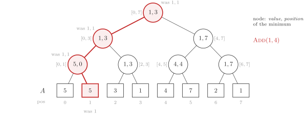
Every node stores the value and the position of the minimum in its range. To combine two children, we take the one with the smaller value, and the left one in case of ties, so that we always report the leftmost minimum. The neutral element is a value of \(+\infty.\) A query rmq(i, j) visits the tree as range_sum does and combines the values of the nodes with a total overlap.

In our running example, the minimum \(1\) occurs at positions \(1,\) \(3\) and \(7,\) so the root stores the value \(1\) and the position \(1.\) For example, rmq(2, 7) combines the nodes \([2,3],\) with minimum \(1\) at position \(3,\) and \([4,7],\) with minimum \(1\) at position \(7:\) the tie is broken in favour of the left one, and the answer is \(3.\)

Now we perform add(1, 4). As for sums, only the nodes on the path from the root to the leaf \(1\) change: the leaf becomes \(5,\) and each node on the path is recomputed from its children. The figure below shows the tree after the update. The minimum of the whole array is now at position \(3.\)

Minimum with Number of Occurrences

Every node stores a pair \((m, c):\) the minimum \(m\) in its range and its number of occurrences \(c.\) Two pairs \((m, c)\) and \((m', c')\) are combined as follows. If \(m = m',\) the result is \((m, c + c').\) Otherwise, the result is the pair with the smaller minimum. The neutral element is \((+\infty, 0).\)

In our running example, the minimum \(1\) occurs \(3\) times, so the root stores \((1, 3).\) The figure below shows the tree after add(1, -1). Now the minimum is \(0\) and it occurs only once.

Searching on a Segment Tree

For example, on our running example search(20) returns \(5,\) since the prefix sums are \(5, 6, 9, 10, 14, 21, 23, 24.\) If \(s\) is larger than the sum of the whole array, which is stored in the root, there is no answer. An add(i, v) with \(v < 0\) is allowed, as long as \(A[i]\) stays non-negative.

Since the values are non-negative, the prefix sums are non-decreasing. Thus, a naive solution is a binary search on the position, which computes a range_sum(0, i) at every step. This takes \(\Theta(\log^2 n)\) time.

We can do better by descending the tree from the root, as in a binary search tree. At a node, let \(s\) be the amount still to reach and let \(x\) be the value of its left child. If \(x \geq s,\) the answer is in the range of the left child, and we move there. Otherwise, the whole left child is in the prefix: we subtract \(x\) from \(s\) and move to the right child. When we reach a leaf, its position is the answer. This descent is correct only with non-negative values: the sum of a range is then at least the sum of any prefix of it, so if the left child does not reach \(s,\) no position inside it can.

The figure below shows search(20). At the root, the left child has sum \(10 < 20,\) so we move right looking for \(20 - 10 = 10.\) At the node \([4,7],\) the left child has sum \(11 \geq 10,\) so we move left. At the node \([4,5],\) the left child has \(4 < 10,\) so we move right looking for \(10-4 = 6.\) We reach the leaf \(5,\) whose value \(7\) covers the remaining \(6,\) and the answer is \(5.\)

We visit one node per level, so search takes \(\Theta(\log n)\) time. The code checks first that the root reaches \(s:\) without this check, the descent would end in the last leaf and return a wrong answer.

impl SegmentTree {
    /// Requires non-negative values. Returns the smallest i such that
    /// A[0] + ... + A[i] >= s, or None if the total sum is smaller than s.
    pub fn search(&self, s: i64) -> Option<usize> {
        if self.tree[0] < s {
            return None; // without this check, the descent would end in the last leaf
        }
        let (mut u, mut l, mut r, mut s) = (0, 0, self.n - 1, s);
        while l < r {
            let m = (l + r) / 2;
            let left = self.tree[2 * u + 1];
            if left >= s {
                u = 2 * u + 1;
                r = m;
            } else {
                s -= left;
                u = 2 * u + 2;
                l = m + 1;
            }
        }
        Some(l)
    }
}

Nodes Storing Data Structures

So far, every node stores a constant number of values. Nothing prevents us from storing a whole data structure in every node. The total space grows, but we can now answer more complex queries.

Counting Occurrences in a Range

Every node stores a hash map that maps each value in its range to its number of occurrences in the range. A query occs(i, j, x) visits the tree as range_sum does. In every node with a total overlap, it looks up \(x\) in the hash map, and the counts are summed. For example, on our running example occs(1, 7, 1) visits the total overlaps \([1,1],\) \([2,3]\) and \([4,7],\) whose counts of the value \(1\) are \(1,\) \(1\) and \(1,\) so the answer is \(3.\)

An add(i, v) changes the value of \(A[i].\) So, in the \(\Theta(\log n)\) hash maps on the path to the leaf \(i,\) we decrement the count of the old value and increment the count of the new one. When a count drops to zero we remove the key, otherwise the hash maps would keep growing with the updates.

Every position of \(A\) appears in the hash maps of the \(\Theta(\log n)\) nodes on its path. So, the space usage is \(\Theta(n \log n).\) Both operations take \(O(\log n)\) time, in expectation, due to the hash maps. For the static version of the problem (no add), a more space-efficient solution is the Wavelet tree.

Successor Queries in a Range

Every node stores the values in its range in a balanced binary search tree. Values may repeat (our running example has three \(1\)s), so the tree must be a multiset: in Rust, a BTreeMap from each value to its number of occurrences. A query successor(i, j, x) visits the tree as range_sum does. In every node with a total overlap, it computes the successor of \(x\) in the binary search tree of the node. The answer is the minimum of these successors, so the neutral element is \(+\infty.\)

The figure below shows the values stored in every node, in sorted order, for our running example, and the query successor(1, 5, 2). It has three total overlaps: \([1,1],\) \([2,3]\) and \([4,5].\) Their successors of \(2\) are \(+\infty,\) \(3\) and \(4,\) so the answer is \(3.\)

We search \(O(\log n)\) binary search trees, and each search takes \(O(\log n)\) time. So, a query takes \(O(\log^2 n)\) time. An add removes one occurrence of the old value and inserts the new one in \(\Theta(\log n)\) binary search trees, in \(O(\log^2 n)\) time. The space usage is \(\Theta(n \log n).\)

If there are no updates, we do not need binary search trees: every node stores its values in a sorted array, which is built in linear time by merging the arrays of its two children, as in merge sort. This structure is often called a merge sort tree, and it is built in \(\Theta(n \log n)\) time. The query time can be further improved to \(O(\log n)\) with a technique called fractional cascading. The idea is that all the searches look for the same \(x,\) so the result of the search in a node can guide the search in its children.

An Application: Counting Increasing Triplets

For example, our running example \(A = [5, 1, 3, 1, 4, 7, 2, 1]\) has \(5\) such triplets of positions: \((1,2,4),\) \((1,2,5),\) \((1,4,5),\) \((2,4,5)\) and \((3,4,5).\) Notice that \((1,3,4)\) is not a triplet, because \(A[1] = A[3]\) and the inequalities are strict.

This application uses only the two basic operations, add and range_sum, so it could be solved with a Fenwick tree as well. Indeed, it uses the same idea as counting inversions with the Fenwick tree: a tree indexed by value, filled during a scan of the array.

What we need to know at each position

Checking all the triplets takes \(\Theta(n^3)\) time. A better idea is to look at the triplets from their middle element. Fix a position \(j,\) and count the triplets whose middle element is \(A[j].\) To build one, we need:

• a position \(i\) to the left of \(j\) with a smaller value, i.e., \(i < j\) and \(A[i] < A[j];\)
• a position \(k\) to the right of \(j\) with a larger value, i.e., \(k > j\) and \(A[k] > A[j].\)

The two choices are independent: any such \(i\) can be combined with any such \(k.\) So, let

• \(L_j\) be the number of positions \(i < j\) with \(A[i] < A[j];\)
• \(R_j\) be the number of positions \(k > j\) with \(A[k] > A[j].\)

Then, exactly \(L_j \cdot R_j\) triplets have \(j\) as their middle position, and we add \(L_j \cdot R_j\) to the result. Every triplet has exactly one middle position, so, summing over all the positions \(j,\) we count every triplet exactly once. The table below shows these numbers for our running example. For instance, for \(j = 4\) we have \(A[4] = 4:\) on its left, the values \(1, 3, 1\) are smaller (\(L_4 = 3\)), and on its right, only the value \(7\) is larger (\(R_4 = 1\)).

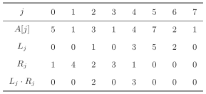
The result is \(2 + 3 = 5,\) as expected. Computing \(L_j\) and \(R_j\) with a scan of the array takes \(\Theta(n)\) time for each \(j,\) so \(\Theta(n^2)\) time overall. Let’s see how two Segment Trees compute each of them in \(O(\log n)\) time.

Two Segment Trees: one for the prefix, one for the suffix

\(L_j\) is a question about the prefix \(A[0..j-1]:\) how many of its values are smaller than \(A[j]\)? Similarly, \(R_j\) is a question about the suffix \(A[j+1..n-1]:\) how many of its values are larger than \(A[j]\)?

To answer such questions, we index a Segment Tree by value, not by position. For now, assume that the values are in \([0, V-1],\) for a small \(V,\) say \(V = O(n)\) (we remove this assumption at the end). In our example, \(V = 8.\) We keep two Segment Trees, each one on an array of \(V\) counters:

• \(P[x]\) is the number of occurrences of the value \(x\) in the prefix \(A[0..j-1];\)
• \(S[x]\) is the number of occurrences of the value \(x\) in the suffix \(A[j+1..n-1].\)

Then, the number of values smaller than \(A[j]\) in the prefix is the sum of the counters \(P[0..A[j]-1],\) and the number of values larger than \(A[j]\) in the suffix is the sum of the counters \(S[A[j]+1..V-1]:\)

• \(L_j\) = range_sum(0, A[j]-1) on \(P;\)
• \(R_j\) = range_sum(A[j]+1, V-1) on \(S.\)

If \(A[j] = 0,\) the first range is empty, and if \(A[j] = V-1,\) the second one is empty. In these cases, we do not call range_sum, which requires a non-empty range, and we take \(0.\)

For example, for \(j = 4\) the prefix is \(5, 1, 3, 1\) and the suffix is \(7, 2, 1.\) The counters are as follows. Since \(A[4] = 4,\) the two queries read \(P[0..3]\) and \(S[5..7],\) whose non-zero counters are in bold.

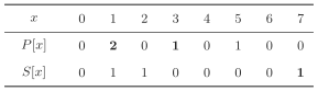
So, \(L_4 = P[0] + P[1] + P[2] + P[3] = 3\) and \(R_4 = S[5] + S[6] + S[7] = 1.\)

It remains to keep \(P\) and \(S\) up to date while \(j\) moves, so that, when we compute \(L_j\) and \(R_j,\) \(P\) describes \(A[0..j-1]\) and \(S\) describes \(A[j+1..n-1].\) We scan \(A\) from left to right. Initially, \(P\) is all zeros, and \(S\) is built from the number of occurrences of every value in the whole array. Then, at every position \(j:\)

1. add(A[j], -1) on \(S:\) the element \(A[j]\) leaves the suffix, which now is \(A[j+1..n-1];\)
2. compute \(L_j\) and \(R_j\) with the two range_sum above, and add \(L_j \cdot R_j\) to the result;
3. add(A[j], 1) on \(P:\) the element \(A[j]\) enters the prefix, which now is \(A[0..j],\) ready for position \(j+1.\)

The \(n\) steps perform two add and two range_sum each, so the scan takes \(\Theta(n \log V)\) time, and the two trees use \(\Theta(V)\) space. Beware that the result can be as large as \(\Theta(n^3),\) e.g., for a sorted array: use a 64-bit integer for it and for the products \(L_j \cdot R_j.\)

What if the values are large, or negative? Only the relative order of the values matters, so we can replace every value with its rank, i.e., its position in the sorted list of the distinct values of \(A.\) Equal values get the same rank, and the order is preserved, so the triplets do not change. To compute the ranks, we sort a copy of \(A,\) remove the duplicates, and find every \(A[j]\) in it with a binary search. In our example, the distinct values are \(1, 2, 3, 4, 5, 7,\) and \(A\) becomes \([4, 0, 2, 0, 3, 5, 1, 0],\) with \(V = 6.\) The ranks are in \([0, n-1],\) so \(V \leq n.\) Computing them takes \(\Theta(n \log n)\) time, and so does the whole algorithm.

Range Updates with Lazy Propagation

The Fenwick tree solves this problem with two Fenwick trees and a clever algebraic trick. The Segment Tree could use exactly the same trick, with two Segment Trees in place of the two Fenwick trees. However, the trick is specific to additions and sums. The Segment Tree has a more general technique, called lazy propagation, which works for many other combinations of range updates and queries, e.g., assigning a value to a range, or adding to a range and asking for the minimum. We will see below what it needs from the operations.

Performing an add for each position in \([i, j]\) takes \(\Theta((j-i+1) \log n)\) time, which is too much for large ranges. The idea of lazy propagation is to be lazy: when a whole node is updated, we update the node and leave a note for its descendants, and we do their work only when a later operation has to go below that node.

So, every node keeps two values: its sum, as before, and a lazy value. The lazy value of a node is an addition that still has to be applied to all the elements below it. We maintain the invariant that the sum stored in a node is always correct; only the nodes below a nonzero lazy value may be out of date.

A range_update(i, j, v) visits the tree as a range_sum(i, j) does.

• Total overlap: all the \(r - l + 1\) elements below the node increase by \(v.\) We add \(v \cdot (r-l+1)\) to its sum and \(v\) to its lazy value, and we stop. Its children are now out of date, but nobody looked at them yet. A leaf has no children, so it does not need a lazy value.
• No overlap: we do nothing.
• Partial overlap: before going down, we push the lazy value of the node to its two children: we apply it to each child as in a total overlap, and we reset it to zero. Then, we recurse on both children, and we recompute the sum of the node from the sums of its children.

The figure below shows range_update(0, 4, 20) on our running example. The node \([0,3]\) has a total overlap: its sum becomes \(10 + 4 \cdot 20 = 90,\) and the update stops there with a lazy value of \(+20.\) The nodes below \([0,3],\) drawn dotted, still store the old values. The leaf \(4\) has a total overlap too, and the sums on its path are recomputed. Below the tree we report the array as it is now.

A range_sum(i, j) works as before, except that it pushes the lazy value of every node with a partial overlap before going down. So, unlike before, a query modifies the tree. The figure below shows range_sum(0, 2) after the update. The node \([0,3]\) has a partial overlap, so it pushes \(+20\) to its children: \([0,1]\) becomes \(6 + 2 \cdot 20 = 46\) and \([2,3]\) becomes \(4 + 2 \cdot 20 = 44,\) and both get a lazy value of \(+20.\) The node \([0,1]\) has a total overlap and returns \(46,\) keeping its lazy value. The node \([2,3]\) has a partial overlap, so it pushes the update to its leaves, which become \(23\) and \(21.\) The answer is \(46 + 23 = 69.\) The subtree of \([4,7]\) is not touched at all.

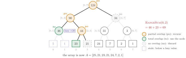
An update pushes too. For example, a later range_update(1, 2, 1) has a partial overlap with \([0,1],\) which still holds the pending \(+20.\) So, it first pushes it, and the leaves \(0\) and \(1\) become \(25\) and \(21.\) Only then the leaf \(1,\) which has a total overlap, becomes \(22.\)

Both operations visit the same nodes as a range_sum and do a constant amount of work in each of them. So, they take \(O(\log n)\) time.

What lazy propagation needs. Lazy propagation is not specific to add and sum. It works whenever (1) we can apply a pending update to the value of a node without looking at its children, and (2) two pending updates can be composed into a single one. For range add and range sum, (1) is “add \(v \cdot (r-l+1)\)” and (2) is “add the two values”. For range add and range minimum, (1) is simply “add \(v\) to the minimum”, because adding \(v\) to every element adds \(v\) to the minimum: in our example, after range_update(0, 4, 20) the minimum of \([0,3]\) goes from \(1\) to \(21\) without touching the children. For a range assignment (“set every entry to \(v\)”), the composition of two pending updates is the later one, and an assignment pushed onto a pending addition replaces it: the order of the updates matters.

/// range_update (add v to every entry in [i, j]) and range_sum.
/// Invariant: tree[u] is always the correct sum of the range of u;
/// lazy[u] is an addition still to be applied to every entry below u.
#[derive(Debug)]
pub struct LazySegmentTree {
    n: usize,
    tree: Vec<i64>,
    lazy: Vec<i64>,
}

impl LazySegmentTree {
    pub fn from_slice(a: &[i64]) -> Self {
        let st = SegmentTree::from_slice(a);
        Self { n: st.n, lazy: vec![0; st.tree.len()], tree: st.tree }
    }

    pub fn range_update(&mut self, i: usize, j: usize, v: i64) {
        assert!(i <= j && j < self.n);
        self.range_update_rec(0, 0, self.n - 1, i, j, v);
    }

    // &mut self: a query may push lazy values down, so it changes the tree.
    pub fn range_sum(&mut self, i: usize, j: usize) -> i64 {
        assert!(i <= j && j < self.n);
        self.range_sum_rec(0, 0, self.n - 1, i, j)
    }

    // Add v to every entry below u, which covers [l, r].
    fn apply(&mut self, u: usize, l: usize, r: usize, v: i64) {
        self.tree[u] += v * (r - l + 1) as i64;
        if l < r {
            self.lazy[u] += v; // a leaf has nothing below it
        }
    }

    // Move the pending addition of u to its children.
    fn push(&mut self, u: usize, l: usize, r: usize) {
        if self.lazy[u] != 0 {
            let m = (l + r) / 2;
            let v = std::mem::take(&mut self.lazy[u]);
            self.apply(2 * u + 1, l, m, v);
            self.apply(2 * u + 2, m + 1, r, v);
        }
    }

    fn range_update_rec(&mut self, u: usize, l: usize, r: usize, i: usize, j: usize, v: i64) {
        if i <= l && r <= j {
            self.apply(u, l, r, v); // total overlap
            return;
        }
        if r < i || j < l {
            return; // no overlap
        }
        self.push(u, l, r); // partial overlap
        let m = (l + r) / 2;
        self.range_update_rec(2 * u + 1, l, m, i, j, v);
        self.range_update_rec(2 * u + 2, m + 1, r, i, j, v);
        self.tree[u] = self.tree[2 * u + 1] + self.tree[2 * u + 2];
    }

    fn range_sum_rec(&mut self, u: usize, l: usize, r: usize, i: usize, j: usize) -> i64 {
        if i <= l && r <= j {
            return self.tree[u];
        }
        if r < i || j < l {
            return 0;
        }
        self.push(u, l, r);
        let m = (l + r) / 2;
        self.range_sum_rec(2 * u + 1, l, m, i, j) + self.range_sum_rec(2 * u + 2, m + 1, r, i, j)
    }
}

Persistent Segment Tree

A data structure is persistent if it keeps all its past versions. Think of time as a counter that starts at \(0.\) Every operation that changes the data structure moves time forward by one. Every query can specify a valid time \(t\) and is answered on the version at time \(t.\) Here, we only update the latest version, while queries can go to any version (partial persistence). With full persistence, we could also update a past version, creating a branch.

In our running example \(A = [5, 1, 3, 1, 4, 7, 2, 1],\) we perform add(3, 10) at time \(1\) and add(7, 2) at time \(2.\) Then, range_sum(0, 7, t) is \(24,\) \(34\) and \(36\) for \(t = 0, 1, 2.\) The ranges matter too: range_sum(2, 3, t) is \(4,\) \(14,\) \(14,\) while range_sum(4, 7, t) is \(14,\) \(14,\) \(16.\)

Attempt #1: Copy Everything

We make a copy of the Segment Tree after every update. A query at time \(t\) is answered on the \(t\)-th copy in \(O(\log n)\) time. However, every add takes \(\Theta(n)\) time to make the copy, and after \(t\) updates the space usage is \(\Theta(n \cdot t).\)

Attempt #2: Keep the History of Every Node

We exploit the fact that an update changes only \(\Theta(\log n)\) nodes. Every node keeps the list of its values, each with the time at which it was set. An add appends a new pair to the list of each of the \(\Theta(\log n)\) nodes on its path. The figure below shows the lists after our two updates, with the pairs coloured by the update that created them. Only the nodes on the two paths have more than one value.

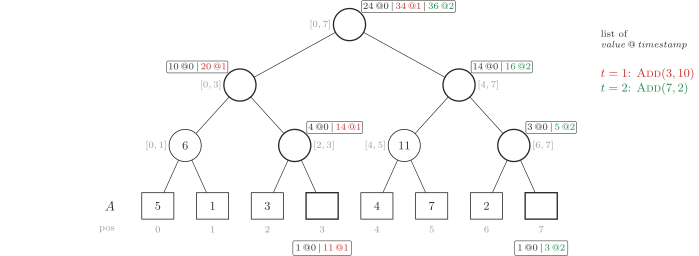
An add takes \(\Theta(\log n)\) time and the space usage is \(\Theta(n + t \log n)\) after \(t\) updates. A query range_sum(i, j, t) visits the tree as before. In every node with a total overlap, it needs the value of the node at time \(t,\) which is the pair with the largest time that is at most \(t.\) This is a predecessor search, which we solve with a binary search on the list. For example, range_sum(2, 3, 1) stops at the node \([2,3],\) whose list is \(4@0 \mid 14@1,\) and returns \(14.\) A query takes \(O(\log n \cdot \log t)\) time.

Attempt #3: Path Copying

We exploit a stronger fact: the \(\Theta(\log n)\) nodes changed by an update lie on a single root-to-leaf path. Instead of modifying these nodes, an add creates a new copy of each of them. The new copy of a node has one child on the path, which is again a new copy, and one child off the path, which is shared with the previous version. We store the root of each version in an array roots, indexed by time.

The figure below shows the two updates of our example, with the range of every internal node. The black nodes are the initial version, the red nodes are created by add(3, 10) and the green ones by add(7, 2). Notice that the green root \([0,7]\) has as its left child the red node \([0,3],\) created by the previous version, and the red root has as its right child the black node \([4,7].\)

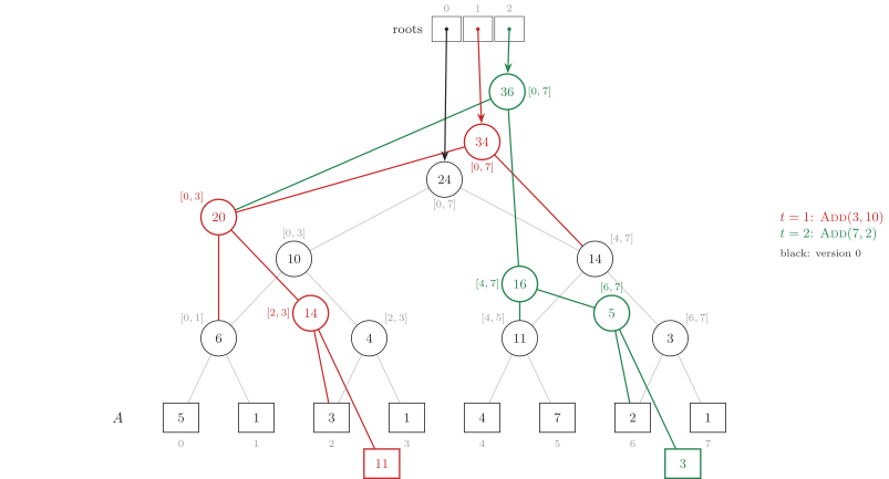
Starting from roots[t], we see exactly the Segment Tree of the version at time \(t.\) So, a query range_sum(i, j, t) is a standard range_sum from roots[t], and it takes \(O(\log n)\) time. An add creates \(\Theta(\log n)\) nodes in \(\Theta(\log n)\) time. After \(t\) updates, the space usage is \(\Theta(n + t \log n).\)

In the implementation, the nodes cannot use the implicit layout anymore, because a node may have several parents. Every node stores the indexes of its children in a vector of nodes.

#[derive(Debug, Clone, Copy)]
struct Node {
    sum: i64,
    left: usize, // index in `nodes`; unused for leaves
    right: usize,
}

/// Every `add` creates a new version; version 0 is the initial array.
#[derive(Debug)]
pub struct PersistentSegmentTree {
    n: usize,
    nodes: Vec<Node>,
    roots: Vec<usize>, // roots[t] is the root of version t
}

impl PersistentSegmentTree {
    pub fn from_slice(a: &[i64]) -> Self {
        assert!(!a.is_empty());
        let mut pst = Self { n: a.len(), nodes: Vec::with_capacity(2 * a.len()), roots: vec![] };
        let root = pst.build(a, 0, a.len() - 1);
        pst.roots.push(root);
        pst
    }

    /// Number of versions (updates performed + 1).
    pub fn versions(&self) -> usize {
        self.roots.len()
    }

    /// A[i] += v on the latest version; returns the new timestamp.
    pub fn add(&mut self, i: usize, v: i64) -> usize {
        assert!(i < self.n);
        let last = *self.roots.last().unwrap();
        let root = self.add_rec(last, 0, self.n - 1, i, v);
        self.roots.push(root);
        self.roots.len() - 1
    }

    /// A[i] + ... + A[j] as it was at time t.
    pub fn range_sum(&self, i: usize, j: usize, t: usize) -> i64 {
        assert!(i <= j && j < self.n && t < self.roots.len());
        self.range_sum_rec(self.roots[t], 0, self.n - 1, i, j)
    }

    fn new_node(&mut self, sum: i64, left: usize, right: usize) -> usize {
        self.nodes.push(Node { sum, left, right });
        self.nodes.len() - 1
    }

    fn build(&mut self, a: &[i64], l: usize, r: usize) -> usize {
        if l == r {
            return self.new_node(a[l], 0, 0);
        }
        let m = (l + r) / 2;
        let left = self.build(a, l, m);
        let right = self.build(a, m + 1, r);
        let sum = self.nodes[left].sum + self.nodes[right].sum;
        self.new_node(sum, left, right)
    }

    // Path copying: a new copy of every node on the root-to-leaf path of i;
    // the child off the path is shared with the previous version.
    fn add_rec(&mut self, u: usize, l: usize, r: usize, i: usize, v: i64) -> usize {
        let Node { sum, mut left, mut right } = self.nodes[u];
        if l == r {
            return self.new_node(sum + v, 0, 0);
        }
        let m = (l + r) / 2;
        if i <= m {
            left = self.add_rec(left, l, m, i, v);
        } else {
            right = self.add_rec(right, m + 1, r, i, v);
        }
        let sum = self.nodes[left].sum + self.nodes[right].sum; // combine
        self.new_node(sum, left, right)
    }

    fn range_sum_rec(&self, u: usize, l: usize, r: usize, i: usize, j: usize) -> i64 {
        if i <= l && r <= j {
            return self.nodes[u].sum;
        }
        if r < i || j < l {
            return 0;
        }
        let m = (l + r) / 2;
        let node = self.nodes[u];
        self.range_sum_rec(node.left, l, m, i, j) + self.range_sum_rec(node.right, m + 1, r, i, j)
    }
}

Why Should We Query the Past?

A typical use of persistence is to turn a sweep into a data structure. If version \(t\) stores the first \(t\) elements of a sequence, a query on version \(t\) is a query on a prefix of the sequence, and the difference between two versions answers a query on a range of the sequence.

Let’s see an example. We want to answer many queries count(i, j, x), each asking for the number of values smaller than \(x\) in \(A[i..j].\) As in the triplets application, we use a Segment Tree indexed by value, on an array \(C\) of \(V\) counters, and we scan \(A\) from left to right with an add(A[t], 1) at every position \(t.\) Version \(t\) is the tree after the first \(t\) additions, so \(C_t[x]\) is the number of occurrences of the value \(x\) in the prefix \(A[0..t-1].\) The occurrences of \(x\) in \(A[i..j]\) are those in the prefix \(A[0..j]\) minus those in the prefix \(A[0..i-1],\) that is, \(C_{j+1}[x] - C_i[x].\) Thus, count(i, j, x) is range_sum(0, x-1, j+1) minus range_sum(0, x-1, i), two queries on two past versions.

In our running example \(A = [5, 1, 3, 1, 4, 7, 2, 1],\) with \(V = 8,\) consider count(2, 6, 4). The range \(A[2..6]\) holds \(3, 1, 4, 7, 2,\) and three of them are smaller than \(4.\) The two versions involved are version \(2,\) after \(5, 1,\) and version \(7,\) after \(5, 1, 3, 1, 4, 7, 2.\)

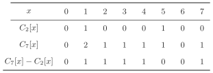
The last row counts the values of \(A[2..6].\) Then, count(2, 6, 4) is

as expected.

Every query costs two range_sum on past versions, so \(O(\log V)\) time. Without persistence, we would have to keep all the \(n+1\) versions of the counters, i.e., \(\Theta(nV)\) space, or to answer the queries offline, sorted by position, during a single scan. With path copying, all the versions take only \(O(V + n \log V)\) space.

The same idea answers harder queries. For example, the \(k\)-th smallest value in \(A[i..j]\) is found by descending the versions \(j+1\) and \(i\) at the same time, as in searching on a Segment Tree. At every node, the difference of the counters of the two left children tells how many values of \(A[i..j]\) fall in the left half. If they are at least \(k,\) we go left; otherwise we go right, after subtracting them from \(k.\) In our example, the \(2\)nd smallest value in \(A[2..6]\) is \(2:\) the left half \([0,3]\) of the root holds three values of the range (\(1, 2, 3\)), so we go left; there, \([0,1]\) holds one value (\(1\)), so we go right, looking for the \(1\)st smallest value in \([2,3],\) which is \(2.\)

Further Readings

• Segment Tree at cp-algorithms
• A Segment Tree tutorial on Codeforces
• Segment Tree at Visualgo
• Lazy propagation in Segment Tree
• Segment tree at Wikipedia. Pay attention: the page also describes a different data structure with the same name, used in computational geometry to store intervals.

Exercises

• Solve Nested Segments with a Segment Tree.
• Circular RMQ: range add and range minimum, with lazy propagation.
• Implement a generic Segment Tree, parametrized by the type of the values, the combine function and the neutral element. Use it for range sums, range minimums and minimum with occurrences. On our running example, you should get range_sum(2, 6) \(= 17,\) rmq(2, 7) \(= 3,\) and a minimum \(1\) with \(3\) occurrences on the whole array.
• Extend search to search(p, s), which returns the smallest position \(i \geq p\) such that \(\sum_{k=p}^{i} A[k] \geq s.\) On our running example, search(2, 8) is \(4.\)
• Implement range add and range minimum with lazy propagation. On our running example, after range_update(0, 4, 20), the minimum of \([0,7]\) is \(1\) and the minimum of \([0,3]\) is \(21.\)
• With a persistent Segment Tree, answer online the queries “how many values of \(A[i..j]\) are at most \(x\)?”. Hint: insert the positions of \(A\) in increasing order of value. On our running example, there are \(3\) values at most \(2\) in \(A[1..6].\)

These notes are for the “Competitive Programming and Contests” course at Università di Pisa.